Decision tree

 Decision tree

·       A decision tree is a tree-based supervised learning method used to predict the output of a target variable.

·       Supervised learning uses labeled data (data with known output variables) to make predictions with the help of regression and classification algorithms.

·       Supervised learning algorithms act as a supervisor for training a model with a defined output variable.

·       It learns from simple decision rules using the various data features.

·       Decision trees in Python can be used to solve both classification and regression problems—they are frequently used in determining odds. 

Useful Concepts

The decision tree algorithm breaks down a dataset into smaller subsets; while during the same time, an associated decision tree is incrementally developed. A decision tree consists of nodes (that test for the value of a certain attribute), edges/branch (that correspond to the outcome of a test and connect to the next node or leaf) & leaf nodes (the terminal nodes that predict the outcome) that makes it a complete structure.

An example of a decision tree can be explained using above binary tree. Let’s say you want to predict whether a person is fit given their information like age, eating habit, and physical activity, etc. The decision nodes here are questions like ‘What’s the age?’, ‘Does he exercise?’, and ‘Does he eat a lot of pizzas’? And the leaves, which are outcomes like either ‘fit’, or ‘unfit’. In this case this was a binary classification problem (a yes no type problem). There are two main types of Decision Trees:

1.       Classification trees (Yes/No types)

A classification tree is an algorithm where the target variable is fixed or categorical. The algorithm is then used to identify the “class” within which a target variable would most likely fall.

An example of a classification-type problem would be determining who will or will not subscribe to a digital platform; or who will or will not graduate from high school.

These are examples of simple binary classifications where the categorical dependent variable can assume only one of two, mutually exclusive values. In other cases, you might have to predict among a number of different variables. For instance, you may have to predict which type of smartphone a consumer may decide to purchase.

In such cases, there are multiple values for the categorical dependent variable. Here’s what a classic classification tree looks like

1.       Regression trees (Continuous data types)

A regression tree refers to an algorithm where the target variable is and the algorithm is used to predict it’s value. As an example of a regression type problem, you may want to predict the selling prices of a residential house, which is a continuous dependent variable.

This will depend on both continuous factors like square footage as well as categorical factors like the style of home, area in which the property is located and so on.

Important Terms Used in Decision Trees

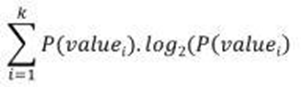
1.         Entropy: Entropy is the measure of uncertainty or randomness in a data set. Entropy handles how a decision tree splits the data.

It is calculated using the following formula:

2.         Information Gain: The information gain measures the decrease in entropy after the data set is split.

It is calculated as follows:

IG( Y, X) = Entropy (Y) - Entropy ( Y | X)

 

3.         Gini Index: The Gini Index is used to determine the correct variable for splitting nodes. It measures how often a randomly chosen variable would be incorrectly identified.

 

4.         Root Node: The root node is always the top node of a decision tree. It represents the entire population or data sample, and it can be further divided into different sets.

 

5.         Decision Node: Decision nodes are sub-nodes that can be split into different sub-nodes; they contain at least two branches.

 

6.         Leaf Node: A leaf node in a decision tree carries the final results. These nodes, which are also known as terminal nodes, cannot be split any further.

How to avoid/counter Overfitting in Decision Trees?

The common problem with Decision trees, especially having a table full of columns, they fit a lot. Sometimes it looks like the tree memorized the training data set. If there is no limit set on a decision tree, it will give you 100% accuracy on the training data set because in the worse case it will end up making 1 leaf for each observation. Thus this affects the accuracy when predicting samples that are not part of the training set.

Here are two ways to remove overfitting:

1.         Pruning Decision Trees.

2.         Random Forest

Pruning Decision Trees:

The splitting process results in fully grown trees until the stopping criteria are reached. But, the fully grown tree is likely to overfit the data, leading to poor accuracy on unseen data.

In pruning, you trim off the branches of the tree, i.e., remove the decision nodes starting from the leaf node such that the overall accuracy is not disturbed. This is done by segregating the actual training set into two sets: training data set, D and validation data set, V. Prepare the decision tree using the segregated training data set, D. Then continue trimming the tree accordingly to optimize the accuracy of the validation data set, V.

In the above diagram, the ‘Age’ attribute in the left-hand side of the tree has been pruned as it has more importance on the right-hand side of the tree, hence removing overfitting.

Random Forest:

Random Forest is an example of ensemble learning, in which we combine multiple machine learning algorithms to obtain better predictive performance.

While implementing the decision tree we will go through the following two phases:

1.         Building Phase

•           Preprocess the dataset.

•           Split the dataset from train and test using Python sklearn package.

•           Train the classifier.

2.         Operational Phase

•           Make predictions.

•           Calculate the accuracy.

ID3:

There are many algorithms out there which construct Decision Trees, but one of the best is called as ID3 Algorithm. ID3 Stands for Iterative Dichotomiser 3. Before discussing the ID3 algorithm, we’ll go through few definitions. Entropy Entropy, also called as Shannon Entropy is denoted by H(S) for a finite set S, is the measure of the amount of uncertainty or randomness in data.

Intuitively, it tells us about the predictability of a certain event. Example, consider a coin toss whose probability of heads is 0.5 and probability of tails is 0.5. Here the entropy is the highest possible, since there’s no way of determining what the outcome might be. Alternatively, consider a coin which has heads on both the sides, the entropy of such an event can be predicted perfectly since we know beforehand that it’ll always be heads. In other words, this event has no randomness hence it’s entropy is zero. In particular, lower values imply less uncertainty while higher values imply high uncertainty. Information Gain Information gain is also called as Kullback-Leibler divergence denoted by IG(S,A) for a set S is the effective change in entropy after deciding on a particular attribute A. It measures the relative change in entropy with respect to the independent variables

IG(S, A) = H (S )- H (S, A)

Alternatively,

n

IG(S, A) = H (S )- å P(x)* H (x)

i=0

where IG(S, A) is the information gain by applying feature A. H(S) is the Entropy of the entire set, while the second term calculates the Entropy after applying the feature A, where P(x) is the probability of event x. Let’s understand this with the help of an example Consider a piece of data collected over the course of 14 days where the features are Outlook, Temperature, Humidity, Wind and the outcome variable is whether Golf was played on the day. Now, our job is to build a predictive model which takes in above 4 parameters and predicts whether Golf will be played on the day. We’ll build a decision tree to do that using ID3 algorithm.

Day	Outlook	Temperature	Humidity	Wind	Play Golf
D1	Sunny	Hot	High	Weak	No
D2	Sunny	Hot	High	Strong	No
D3	Overcast	Hot	High	Weak	Yes
D4	Rain	Mild	High	Weak	Yes
D5	Rain	Cool	Normal	Weak	Yes
D6	Rain	Cool	Normal	Strong	No
D7	Overcast	Cool	Normal	Strong	Yes
D8	Sunny	Mild	High	Weak	No
D9	Sunny	Cool	Normal	Weak	Yes
D10	Rain	Mild	Normal	Weak	Yes
D11	Sunny	Mild	Normal	Strong	Yes
D12	Overcast	Mild	High	Strong	Yes
D13	Overcast	Hot	Normal	Weak	Yes
D14	Rain	Mild	High	Strong	No